Styling visual attributes

Using themes

Bokeh’s themes are a set of pre-defined design parameters that you can apply to your plots. Themes can include settings for parameters such as colors, fonts, or line styles.

Applying Bokeh’s built-in themes

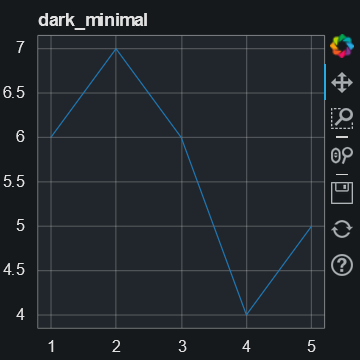
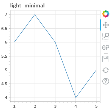
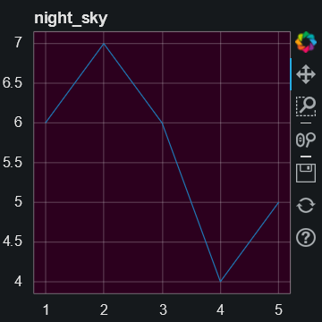
Bokeh comes with five built-in themes to quickly change the appearance of one or more plots: caliber, dark_minimal, light_minimal, night_sky, and contrast.

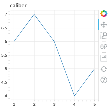
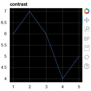
To use one of the built-in themes, assign the name of the theme you want to use to the theme property of your document.

For example:

from bokeh.io import curdoc
from bokeh.plotting import figure, output_file, show

x = [1, 2, 3, 4, 5]
y = [6, 7, 6, 4, 5]

output_file("dark_minimal.html")

curdoc().theme = 'dark_minimal'

p = figure(title='dark_minimal', width=300, height=300)
p.line(x, y)

show(p)

For more examples and detailed information, see bokeh.themes.

Creating custom themes

Themes in Bokeh are defined in YAML or JSON files. To create your own theme files, follow the format defined in bokeh.themes.Theme.

Using YAML, for example:

attrs:
    Figure:
        background_fill_color: '#2F2F2F'
        border_fill_color: '#2F2F2F'
        outline_line_color: '#444444'
    Axis:
        axis_line_color: !!null
    Grid:
        grid_line_dash: [6, 4]
        grid_line_alpha: .3
    Title:
        text_color: "white"

To use your custom theme in a Bokeh plot, load your YAML or JSON file into a bokeh.themes.Theme object:

from bokeh.themes import Theme
curdoc().theme = Theme(filename="./theme.yml")

Using palettes

Palettes are sequences of RGB(A) hex strings that define a colormap. The sequences you use for defining colormaps can be either lists or tuples. Once you have created a colormap, you can use it with the color attribute of many plot objects from bokeh.plotting.

Bokeh includes several pre-defined palettes, such as the standard Brewer palettes. To use one of those pre-defined palettes, import it from the bokeh.palettes module. When you import “Spectral6”, for example, Bokeh gives you access to a six element list of RGB(A) hex strings from the Brewer “Spectral” colormap:

>>> from bokeh.palettes import Spectral6
>>> Spectral6
['#3288bd', '#99d594', '#e6f598', '#fee08b', '#fc8d59', '#d53e4f']

For a list of all the standard palettes included in Bokeh, see bokeh.palettes.

You can also create custom palettes by defining a sequence of RGB(A) hex strings yourself.

Using mappers

Use Bokeh’s color mappers to encode a sequence of data into a palette of colors that are based on the values in that sequence. You can then set a marker object’s color attribute to your color mapper. Bokeh includes several types of mappers to encode colors:

• factor_cmap(): Maps colors to specific categorical elements. See Handling categorical data for more detail.

• linear_cmap(): Maps a range of numeric values across the available colors from high to low. For example, a range of [0,99] given the colors [‘red’, ‘green’, ‘blue’] would be mapped as follows:

      x < 0  : 'red'     # values < low are clamped
  0 >= x < 33 : 'red'
  33 >= x < 66 : 'green'
  66 >= x < 99 : 'blue'
  99 >= x      : 'blue'    # values > high are clamped
  

• log_cmap(): Similar to linear_cmap but uses a natural log scale to map the colors.

These mapper functions return a DataSpec property. Pass this property to the color attribute of the glyph you want to use it with.

The dataspec that the mapper function returns includes a bokeh.transform. You can access this data to use the result of the mapper function in a different context. To create a ColorBar, for example:

from bokeh.models import ColorBar, ColumnDataSource
from bokeh.palettes import Spectral6
from bokeh.plotting import figure, output_file, show
from bokeh.transform import linear_cmap

output_file("styling_linear_mappers.html", title="styling_linear_mappers.py example")

x = [1,2,3,4,5,7,8,9,10]
y = [1,2,3,4,5,7,8,9,10]

#Use the field name of the column source
mapper = linear_cmap(field_name='y', palette=Spectral6 ,low=min(y) ,high=max(y))

source = ColumnDataSource(dict(x=x,y=y))

p = figure(width=300, height=300, title="Linear Color Map Based on Y")

p.circle(x='x', y='y', line_color=mapper,color=mapper, fill_alpha=1, size=12, source=source)

color_bar = ColorBar(color_mapper=mapper['transform'], width=8)

p.add_layout(color_bar, 'right')

show(p)

Customizing visual properties

To style the visual attributes of Bokeh plots, you need to know what the available properties are. The full reference guide contains all properties of every object individually. However, there are three groups of properties that many objects have in common. They are:

• line properties: line color, width, etc.

• fill properties: fill color, alpha, etc.

• text properties: font styles, colors, etc.

This section contains more details about some of the most common properties.

Line properties

line_color

color to use to stroke lines with

line_width

line stroke width in units of pixels

line_alpha

floating point between 0 (transparent) and 1 (opaque)

line_join

how path segments should be joined together

• 'miter'

• 'round'

• 'bevel'

line_cap

how path segments should be terminated

• 'butt'

• 'round'

• 'square'

line_dash

a line style to use

• 'solid'

• 'dashed'

• 'dotted'

• 'dotdash'

• 'dashdot'

• an array of integer pixel distances that describe the on-off pattern of dashing to use

• a string of spaced integers matching the regular expression ‘^(\d+(\s+\d+)*)?$’ that describe the on-off pattern of dashing to use

line_dash_offset

the distance in pixels into the line_dash that the pattern should start from

Fill properties

fill_color

color to use to fill paths with

fill_alpha

floating point between 0 (transparent) and 1 (opaque)

Hatch properties

hatch_color

color to use to stroke hatch patterns with

hatch_alpha

floating point between 0 (transparent) and 1 (opaque)

hatch_weight

line stroke width in units of pixels

hatch_scale

a rough measure of the “size” of a pattern. This value has different specific meanings, depending on the pattern.

hatch_pattern

a string name (or abbreviation) for a built-in pattern, or a string name of a pattern provided in hatch_extra. The built-in patterns are:

Built-in Hatch Patterns

FullName	Abbreviation	Example
blank	" "
dot	"."
ring	"o"
horizontal_line	"-"
vertical_line	"|"
cross	"+"
horizontal_dash	'"'
vertical_dash	":"
spiral	"@"
right_diagonal_line	"/"
left_diagonal_line	"\\"
diagonal_cross	"x"
right_diagonal_dash	","
left_diagonal_dash	"`"
horizontal_wave	"v"
vertical_wave	">"
criss_cross	"*"

hatch_extra

a dict mapping string names to custom pattern implementations. The name can be referred to by hatch_pattern. For example, if the following value is set for hatch_extra:

hatch_extra={ 'mycustom': ImageURLTexture(url=...) }

then the name "mycustom" may be set as a hatch_pattern.

Text properties

text_font

font name, e.g., 'times', 'helvetica'

text_font_size

font size in px, em, or pt, e.g., '16px', '1.5em'

text_font_style

font style to use

• 'normal' normal text

• 'italic' italic text

• 'bold' bold text

text_color

color to use to render text with

text_alpha

floating point between 0 (transparent) and 1 (opaque)

text_align

horizontal anchor point for text: 'left', 'right', 'center'

text_baseline

vertical anchor point for text

• 'top'

• 'middle'

• 'bottom'

• 'alphabetic'

• 'hanging'

Note

There is currently only support for filling text. An interface to stroke the outlines of text has not yet been exposed.

Visible property

Glyph renderers, axes, grids, and annotations all have a visible property. Use this property to turn them on and off.

from bokeh.io import output_file, show
from bokeh.plotting import figure

# We set-up a standard figure with two lines
p = figure(width=500, height=200, tools='')
visible_line = p.line([1, 2, 3], [1, 2, 1], line_color="blue")
invisible_line = p.line([1, 2, 3], [2, 1, 2], line_color="pink")

# We hide the xaxis, the xgrid lines, and the pink line
invisible_line.visible = False
p.xaxis.visible = False
p.xgrid.visible = False

output_file("styling_visible_property.html")

show(p)

This can be particularly useful in interactive examples with a Bokeh server or CustomJS.

from bokeh.io import output_file, show
from bokeh.layouts import layout
from bokeh.models import BoxAnnotation, Toggle
from bokeh.plotting import figure

output_file("styling_visible_annotation_with_interaction.html")

p = figure(width=600, height=200, tools='')
p.line([1, 2, 3], [1, 2, 1], line_color="blue")
pink_line = p.line([1, 2, 3], [2, 1, 2], line_color="pink")

green_box = BoxAnnotation(left=1.5, right=2.5, fill_color='green', fill_alpha=0.1)
p.add_layout(green_box)

# Use js_link to connect button active property to glyph visible property

toggle1 = Toggle(label="Green Box", button_type="success", active=True)
toggle1.js_link('active', green_box, 'visible')

toggle2 = Toggle(label="Pink Line", button_type="success", active=True)
toggle2.js_link('active', pink_line, 'visible')

show(layout([p], [toggle1, toggle2]))

Color properties

Bokeh objects have several properties related to colors. Use those color properties to control the appearance of lines, fills, or text, for example.

Use one of these options to define colors in Bokeh:

• Any of the named CSS colors, such as 'green' or 'indigo'. You can also use the additional name 'transparent' (equal to '#00000000').

• An RGB(A) hex value, such as '#FF0000' (without alpha information) or '#44444444' (with alpha information).

• A CSS4 rgb(), rgba(), or hsl() color string, such as 'rgb(0 127 0 / 1.0)', 'rgba(255, 0, 127, 0.6)', or 'hsl(60deg 100% 50% / 1.0)'.

• A 3-tuple of integers (r, g, b) (where r, g, and b are integers between 0 and 255).

• A 4-tuple of (r, g, b, a) (where r, g, and b are integers between 0 and 255 and a is a floating-point value between 0 and 1).

• A 32-bit unsigned integer representing RGBA values in a 0xRRGGBBAA byte order pattern, such as 0xffff00ff or 0xff0000ff.

To define a series of colors, use an array of color data such as a list or the column of a ColumnDataSource. This also includes NumPy arrays.

For example:

import numpy as np

from bokeh.plotting import figure, output_file, show

output_file("specifying_colors.html")

x = [1, 2, 3]
y1 = [1, 4, 2]
y2 = [2, 1, 4]
y3 = [4, 3, 2]

# use a single RGBA color
single_color = (255, 0, 0, 0.5)

# use a list of different colors
list_of_colors = [
    "hsl(60deg 100% 50% / 1.0)",
    "rgba(0, 0, 255, 0.9)",
    "LightSeaGreen",
]

# use a series of color values as numpy array
numpy_array_of_colors = np.array(
    [
        0xFFFF00FF,
        0x00FF00FF,
        0xFF000088,
    ],
    np.uint32,
)

p = figure(title="Specifying colors")

# add glyphs to plot
p.line(x, y1, line_color=single_color)
p.circle(x, y2, radius=0.12, color=list_of_colors)
p.triangle(x, y3, size=30, fill_color=numpy_array_of_colors)

show(p)

In addition to specifying the alpha value of a color when defining the color itself, you can also set an alpha value separately by using the line_alpha or fill_alpha properties of a glyph.

In case you define a color with an alpha value and also explicitly provide an alpha value through a line_alpha or fill_alpha property at the same time, the following happens: If your color definition does include an alpha value (such as '#00FF0044' or 'rgba(255, 0, 127, 0.6)'), this alpha value takes precedence over the alpha value you provide through the objects’s property. Otherwise, the alpha value defined in the objects’s property is used.

The following figure demonstrates each possible combination of using RGB and RGBA colors together with the line_alpha or fill_alpha properties:

Note

If you use Bokeh’s plotting interface, you also have the option to specify color and/or alpha as keywords when calling a renderer method. Bokeh automatically applies these values to the corresponding fill and line properties of your glyphs.

You then still have the option to provide additional fill_color, fill_alpha, line_color, and line_alpha arguments as well. In this case, the former will take precedence.

Screen units and data-space units

When setting visual properties of Bokeh objects, you use either screen units or data-space units:

• Screen units use raw numbers of pixels to specify height or width

• Data-space units are relative to the data and the axes of the plot

Take a 400 pixel by 400 pixel graph with x and y axes ranging from 0 through 10, for example. A glyph that is one fifth as wide and tall as the graph would have a size of 80 screen units or 2 data-space units.

Objects in Bokeh that support both screen units and data-space units usually have a dedicated property to choose which unit to use. This unit-setting property is the name of the property with an added _units. For example: A Whisker annotation has the property upper. To define which unit to use, set the upper_units property to either 'screen' or 'data'.

Selecting plot objects

If you want to customize the appearance of any element of your Bokeh plot, you first need to identify which object you want to modify. As described in Defining key concepts, Bokeh plots are a combination of Python objects that represent all the different parts of your plot: its grids, axes, and glyphs, for example.

Some objects have convenience methods to help you identify the objects you want to address. See Styling axes, Styling grids, and Styling legends for examples.

To query for any Bokeh plot object, use the select() method on Plot. For example, to find all PanTool objects in a plot:

>>> p.select(type=PanTool)
[<bokeh.models.tools.PanTool at 0x106608b90>]

You can also use the select() method to query on other attributes as well:

>>> p.circle(0, 0, name="mycircle")
<bokeh.plotting.Figure at 0x106608810>

>>> p.select(name="mycircle")
[<bokeh.models.renderers.GlyphRenderer at 0x106a4c810>]

This query method can be especially useful when you want to style visual attributes of Styling glyphs.

Styling plots

In addition to the individual plot elements, a Plot object itself also has several visual characteristics that you can customize: the dimensions of the plot, its backgrounds, borders, or outlines, for example. This section describes how to change these attributes of a Bokeh plot.

The example code primarily uses the bokeh.plotting interface to create plots. However, the instructions apply regardless of how a Bokeh plot was created.

Dimensions

To change the width and height of a Plot, use its width and height attributes. Those two attributes use screen units. They control the size of the entire canvas area, including any axes or titles (but not the toolbar).

If you are using the bokeh.plotting interface, you can pass these values to figure() directly:

from bokeh.plotting import figure, output_file, show

output_file("dimensions.html")

# create a new plot with specific dimensions
p = figure(width=700)
p.height = 300

p.circle([1, 2, 3, 4, 5], [2, 5, 8, 2, 7], size=10)

show(p)

Responsive sizes

To automatically adjust the width or height of your plot in relation to the available space in the browser, use the plot’s sizing_mode property.

To control how the plot scales to fill its container, see the documentation for layouts, in particular the sizing_mode property of LayoutDOM.

If you set sizing_mode to anything different than fixed, Bokeh adjusts the width and height as soon as a plot is rendered. However, Bokeh uses width and height to calculate the initial aspect ratio of your plot.

Plots will only resize down to a minimum of 100px (height or width) to prevent problems in displaying your plot.

Title

To style the title of your plot, use the Title annotation, which is available as the .title property of the Plot.

You can use most of the standard text properties. However, text_align and text_baseline do not apply. To position the title relative to the entire plot, use the properties align and offset instead.

As an example, to set the color and font style of the title text, use plot.title.text_color:

from bokeh.plotting import figure, output_file, show

output_file("title.html")

p = figure(width=400, height=400, title="Some Title")
p.title.text_color = "olive"
p.title.text_font = "times"
p.title.text_font_style = "italic"

p.circle([1, 2, 3, 4, 5], [2, 5, 8, 2, 7], size=10)

show(p)

Background

To change the background fill style, adjust the background_fill_color and background_fill_alpha properties of the Plot object:

from bokeh.plotting import figure, output_file, show

output_file("background.html")

p = figure(width=400, height=400)
p.background_fill_color = "beige"
p.background_fill_alpha = 0.5

p.circle([1, 2, 3, 4, 5], [2, 5, 8, 2, 7], size=10)

show(p)

Border

To adjust the border fill style, use the border_fill_color and border_fill_alpha properties of the Plot object. You can also set the minimum border on each side (in screen units) with these properties:

• min_border_left

• min_border_right

• min_border_top

• min_border_bottom

Additionally, if you set min_border, Bokeh applies a minimum border setting to all sides as a convenience. The min_border default value is 40px.

from bokeh.plotting import figure, output_file, show

output_file("border.html")

p = figure(width=400, height=400)
p.border_fill_color = "whitesmoke"
p.min_border_left = 80

p.circle([1,2,3,4,5], [2,5,8,2,7], size=10)

show(p)

Outline

Bokeh Plot objects have various line properties. To change the appearance of outlines, use those line properties that are prefixed with outline_.

For example, to set the color of the outline, use outline_line_color:

from bokeh.plotting import figure, output_file, show

output_file("outline.html")

p = figure(width=400, height=400)
p.outline_line_width = 7
p.outline_line_alpha = 0.3
p.outline_line_color = "navy"

p.circle([1,2,3,4,5], [2,5,8,2,7], size=10)

show(p)

Styling glyphs

To style the fill, line, or text properties of a glyph, you first need to identify which GlyphRenderer you want to customize. If you are using the bokeh.plotting interface, the glyph functions return the renderer:

>>> r = p.circle([1,2,3,4,5], [2,5,8,2,7])
>>> r
<bokeh.models.renderers.GlyphRenderer at 0x106a4c810>

Next, obtain the glyph itself from the .glyph attribute of a GlyphRenderer:

>>> r.glyph
<bokeh.models.glyphs.Circle at 0x10799ba10>

This is the object to set fill, line, or text property values for:

from bokeh.plotting import figure, output_file, show

output_file("axes.html")

p = figure(width=400, height=400)
r = p.circle([1,2,3,4,5], [2,5,8,2,7])

glyph = r.glyph
glyph.size = 60
glyph.fill_alpha = 0.2
glyph.line_color = "firebrick"
glyph.line_dash = [6, 3]
glyph.line_width = 2

show(p)

Selected and unselected glyphs

To customize the styling of selected and non-selected glyphs, set the selection_glyph and nonselection_glyph attributes of the GlyphRenderer. You can either set them manually or by passing them to add_glyph().

The plot below uses the bokeh.plotting interface to set these attributes. Click or tap any of the circles on the plot to see the effect on the selected and non-selected glyphs. To clear the selection and restore the original state, click anywhere in the plot outside of a circle.

from bokeh.io import output_file, show
from bokeh.models import Circle
from bokeh.plotting import figure

output_file("styling_selections.html")

plot = figure(width=400, height=400, tools="tap", title="Select a circle")
renderer = plot.circle([1, 2, 3, 4, 5], [2, 5, 8, 2, 7], size=50)

selected_circle = Circle(fill_alpha=1, fill_color="firebrick", line_color=None)
nonselected_circle = Circle(fill_alpha=0.2, fill_color="blue", line_color="firebrick")

renderer.selection_glyph = selected_circle
renderer.nonselection_glyph = nonselected_circle

show(plot)

If you just need to set the color or alpha parameters of the selected or non-selected glyphs, provide color and alpha arguments to the glyph function, prefixed by "selection_" or "nonselection_":

from bokeh.io import output_file, show
from bokeh.plotting import figure

output_file("styling_selections.html")

plot = figure(width=400, height=400, tools="tap", title="Select a circle")
renderer = plot.circle([1, 2, 3, 4, 5], [2, 5, 8, 2, 7], size=50,

                       # set visual properties for selected glyphs
                       selection_color="firebrick",

                       # set visual properties for non-selected glyphs
                       nonselection_fill_alpha=0.2,
                       nonselection_fill_color="blue",
                       nonselection_line_color="firebrick",
                       nonselection_line_alpha=1.0)

show(plot)

If you use the bokeh.models interface, use the add_glyph() function:

p = Plot()
source = ColumnDataSource(dict(x=[1, 2, 3], y=[1, 2, 3]))

initial_circle = Circle(x='x', y='y', fill_color='blue', size=50)
selected_circle = Circle(fill_alpha=1, fill_color="firebrick", line_color=None)
nonselected_circle = Circle(fill_alpha=0.2, fill_color="blue", line_color="firebrick")

p.add_glyph(source,
            initial_circle,
            selection_glyph=selected_circle,
            nonselection_glyph=nonselected_circle)

Note

When rendering, Bokeh considers only the visual properties of selection_glyph and nonselection_glyph. Changing positions, sizes, etc., will have no effect.

Hover inspections

To style the appearance of glyphs that are hovered over, pass color or alpha parameters prefixed with "hover_" to your renderer function.

Alternatively, set the selection_glyph and nonselection_glyph attributes of the GlyphRenderer, just like in Selected and unselected glyphs above.

This example uses the first method of passing a color parameter with the "hover_" prefix:

from bokeh.models import HoverTool
from bokeh.plotting import figure, output_file, show
from bokeh.sampledata.glucose import data

output_file("styling_hover.html")

subset = data.loc['2010-10-06']

x, y = subset.index.to_series(), subset['glucose']

# Basic plot setup
plot = figure(width=600, height=300, x_axis_type="datetime", tools="",
              toolbar_location=None, title='Hover over points')

plot.line(x, y, line_dash="4 4", line_width=1, color='gray')

cr = plot.circle(x, y, size=20,
                fill_color="grey", hover_fill_color="firebrick",
                fill_alpha=0.05, hover_alpha=0.3,
                line_color=None, hover_line_color="white")

plot.add_tools(HoverTool(tooltips=None, renderers=[cr], mode='hline'))

show(plot)

Note

When rendering, Bokeh considers only the visual properties of hover_glyph. Changing positions, sizes, etc. will have no effect.

Styling tool overlays

Some Bokeh tools also have configurable visual attributes.

For instance, the various region selection tools and the box zoom tool all have an overlay. To style their line and fill properties, pass values to the respective attributes:

import numpy as np

from bokeh.models import BoxSelectTool, BoxZoomTool, LassoSelectTool
from bokeh.plotting import figure, output_file, show

output_file("styling_tool_overlays.html")

x = np.random.random(size=200)
y = np.random.random(size=200)

# Basic plot setup
plot = figure(width=400, height=400, title='Select and Zoom',
              tools="box_select,box_zoom,lasso_select,reset")

plot.circle(x, y, size=5)

select_overlay = plot.select_one(BoxSelectTool).overlay

select_overlay.fill_color = "firebrick"
select_overlay.line_color = None

zoom_overlay = plot.select_one(BoxZoomTool).overlay

zoom_overlay.line_color = "olive"
zoom_overlay.line_width = 8
zoom_overlay.line_dash = "solid"
zoom_overlay.fill_color = None

plot.select_one(LassoSelectTool).overlay.line_dash = [10, 10]

show(plot)

For more information, see the reference guide’s entries for BoxSelectTool.overlay, BoxZoomTool.overlay, LassoSelectTool.overlay, PolySelectTool.overlay, and RangeTool.overlay.

Toggling ToolBar autohide

To make your toolbar hide automatically, set the toolbar’s autohide property to True. When you set autohide to True, the toolbar is visible only when the mouse is inside the plot area and is otherwise hidden.

from bokeh.plotting import figure, output_file, show

output_file("styling_toolbar_autohide.html")

# Basic plot setup
plot = figure(width=400, height=400, title='Toolbar Autohide')
plot.line([1,2,3,4,5], [2,5,8,2,7])

# Set autohide to true to only show the toolbar when mouse is over plot
plot.toolbar.autohide = True

show(plot)

Styling axes

This section focuses on changing various visual properties of Bokeh plot axes.

To set style attributes on Axis objects, use the xaxis, yaxis, and axis methods on Plot to first obtain a plot’s Axis objects. For example:

>>> p.xaxis
[<bokeh.models.axes.LinearAxis at 0x106fa2390>]

Because there may be more than one axis, this method returns a list of Axis objects. However, as a convenience, these lists are splattable. This means that you can set attributes directly on this result, and the attributes will be applied to all the axes in the list. For example:

p.xaxis.axis_label = "Temperature"

This changes the value of axis_label for every x-axis of p, however many there may be.

The example below demonstrates the use of the xaxis, yaxis, and axis methods in more details:

from bokeh.plotting import figure, output_file, show

output_file("axes.html")

p = figure(width=400, height=400)
p.circle([1,2,3,4,5], [2,5,8,2,7], size=10)

# change just some things about the x-axis
p.xaxis.axis_label = "Temp"
p.xaxis.axis_line_width = 3
p.xaxis.axis_line_color = "red"

# change just some things about the y-axis
p.yaxis.axis_label = "Pressure"
p.yaxis.major_label_text_color = "orange"
p.yaxis.major_label_orientation = "vertical"

# change things on all axes
p.axis.minor_tick_in = -3
p.axis.minor_tick_out = 6

show(p)

Labels

To add or change the text of an axis’ overall label, use the axis_label property. To add line breaks to the text in an axis label, include \n in your string.

To control the visual appearance of the label text, use any of the standard text properties prefixed with axis_label_. For instance, to set the text color of the label, set axis_label_text_color.

To change the distance between the axis label and the major tick labels, set the axis_label_standoff property.

For example:

from bokeh.plotting import figure, output_file, show

output_file("bounds.html")

p = figure(width=400, height=400)
p.circle([1,2,3,4,5], [2,5,8,2,7], size=10)

p.xaxis.axis_label = "Lot Number"
p.xaxis.axis_label_text_color = "#aa6666"
p.xaxis.axis_label_standoff = 30

p.yaxis.axis_label = "Bin Count"
p.yaxis.axis_label_text_font_style = "italic"

show(p)

Bounds

To limit the bounds where axes are drawn, set the bounds property of an axis object to a 2-tuple of (start, end):

from bokeh.plotting import figure, output_file, show

output_file("bounds.html")

p = figure(width=400, height=400)
p.circle([1,2,3,4,5], [2,5,8,2,7], size=10)

p.xaxis.bounds = (2, 4)

show(p)

Tick locations

Bokeh uses several “ticker” models to decide where to display ticks on axes (categorical, datetime, mercator, linear, or log scale). To configure the placements of ticks, use the .ticker property of an axis.

If you use the bokeh.plotting interface, Bokeh chooses an appropriate ticker placement model automatically.

In case you need to control which ticker placement model to use, you can also explicitly define a list of tick locations. Assign FixedTicker with a list of tick locations to an axis:

from bokeh.plotting import figure
from bokeh.models.tickers import FixedTicker

p = figure()

# no additional tick locations will be displayed on the x-axis
p.xaxis.ticker = FixedTicker(ticks=[10, 20, 37.4])

As a shortcut, you can also supply the list of ticks directly to an axis’ ticker property:

from bokeh.plotting import figure, output_file, show

output_file("fixed_ticks.html")

p = figure(width=400, height=400)
p.circle([1,2,3,4,5], [2,5,8,2,7], size=10)

p.xaxis.ticker = [2, 3.5, 4]

show(p)

Tick lines

To control the visual appearance of the major and minor ticks, set the appropriate line properties, prefixed with major_tick_ and minor_tick_, respectively.

For instance, to set the color of the major ticks, use major_tick_line_color. To hide either set of ticks, set the color to None.

Additionally, to control how far in and out of the plotting area the ticks extend, use the properties major_tick_in/major_tick_out and minor_tick_in/minor_tick_out. These values are in screen units. Therefore, you can use negative values.

from bokeh.plotting import figure, output_file, show

output_file("axes.html")

p = figure(width=400, height=400)
p.circle([1,2,3,4,5], [2,5,8,2,7], size=10)

p.xaxis.major_tick_line_color = "firebrick"
p.xaxis.major_tick_line_width = 3
p.xaxis.minor_tick_line_color = "orange"

p.yaxis.minor_tick_line_color = None

p.axis.major_tick_out = 10
p.axis.minor_tick_in = -3
p.axis.minor_tick_out = 8

show(p)

Tick label formats

To style the text of axis labels, use the TickFormatter object of the axis’ formatter property. Bokeh uses a number of ticker formatters by default in different situations:

• BasicTickFormatter — Default formatter for linear axes.

• CategoricalTickFormatter — Default formatter for categorical axes.

• DatetimeTickFormatter — Default formatter for datetime axes.

• LogTickFormatter — Default formatter for log axes.

These default tick formatters do not expose many configurable properties. To control tick formatting at a finer-grained level, use one of the NumeralTickFormatter or PrintfTickFormatter described below.

Note

To replace a tick formatter on an axis, you must set the formatter property on an actual Axis object, not on a splattable list. This is why the following examples use p.yaxis[0].formatter, etc. (with the subscript [0]).

NumeralTickFormatter

The NumeralTickFormatter has a format property that can be used to control the text formatting of axis ticks.

from bokeh.models import NumeralTickFormatter
from bokeh.plotting import figure, output_file, show

output_file("gridlines.html")

p = figure(width=400, height=400)
p.circle([1,2,3,4,5], [2,5,8,2,7], size=10)

p.xaxis[0].formatter = NumeralTickFormatter(format="0.0%")
p.yaxis[0].formatter = NumeralTickFormatter(format="$0.00")

show(p)

Many additional formats are available. See the full NumeralTickFormatter documentation in the reference guide.

PrintfTickFormatter

The PrintfTickFormatter has a format property that can be used to control the text formatting of axis ticks using printf style format strings.

from bokeh.models import PrintfTickFormatter
from bokeh.plotting import figure, output_file, show

output_file("gridlines.html")

p = figure(width=400, height=400)
p.circle([1,2,3,4,5], [2,5,8,2,7], size=10)

p.xaxis[0].formatter = PrintfTickFormatter(format="%4.1e")
p.yaxis[0].formatter = PrintfTickFormatter(format="%5.3f mu")

show(p)

For full details about formats, see the full PrintfTickFormatter documentation in the reference guide.

FuncTickFormatter

To fully customize the format of axis ticks, use the FuncTickFormatter in combination with a JavaScript snippet as its code property.

The variable tick contains the unformatted tick value. It is accessible in the snippet or function namespace at render time:

from bokeh.models import FuncTickFormatter
from bokeh.plotting import figure, output_file, show

output_file("formatter.html")

p = figure(width=500, height=500)
p.circle([0, 2, 4, 6, 8, 10], [6, 2, 4, 10, 8, 0], size=30)

p.yaxis.formatter = FuncTickFormatter(code="""
    return Math.floor(tick) + " + " + (tick % 1).toFixed(2)
""")

show(p)

Tick label orientation

To control the orientation of major tick labels, use the major_label_orientation property. This property accepts the values "horizontal" or "vertical" or a floating-point number that gives the angle (in radians) to rotate from the horizontal:

from math import pi

from bokeh.plotting import figure, output_file, show

output_file("gridlines.html")

p = figure(width=400, height=400)
p.circle([1,2,3,4,5], [2,5,8,2,7], size=10)

p.xaxis.major_label_orientation = pi/4
p.yaxis.major_label_orientation = "vertical"

show(p)

Note

There are more properties that you can use to configure Bokeh axes. For a complete list of all the various attributes that you can set on different types of Bokeh axes, see the axes section of the reference guide.

Styling grids

In this section, you will learn how to set the visual properties of grid lines and grid bands on Bokeh plots.

To obtain a plot’s Grid objects, use the xgrid, ygrid, and grid methods on Plot. This works similar to the convenience methods for axes:

>>> p.grid
[<bokeh.models.grids.Grid at 0x106fa2278>,
 <bokeh.models.grids.Grid at 0x106fa22e8>]

These methods also return splattable lists. You can set an attribute on the list as if it was a single object, and the attribute is changed for every element of the list:

p.grid.line_dash = [4 2]

Note

The xgrid property provides the grid objects that intersect the x-axis (meaning vertically oriented objects). Correspondingly, ygrid provides the grid objects that intersect the y-axis (meaning horizontally oriented objects).

Lines

To configure the visual appearance of grid lines, use a collection of line properties, prefixed with grid_.

For instance, to set the color of grid lines, use grid_line_color. To hide grid lines, set their line color to None:

from bokeh.plotting import figure, output_file, show

output_file("gridlines.html")

p = figure(width=400, height=400)
p.circle([1,2,3,4,5], [2,5,8,2,7], size=10)

# change just some things about the x-grid
p.xgrid.grid_line_color = None

# change just some things about the y-grid
p.ygrid.grid_line_alpha = 0.5
p.ygrid.grid_line_dash = [6, 4]

show(p)

Minor lines

To configure the visual appearance of minor grid lines, use a collection of line properties, prefixed with minor_grid_.

For instance, to set the color of grid lines, use minor_grid_line_color. By default, minor grid lines are hidden (which means that their line color is set to None):

from bokeh.plotting import figure, output_file, show

output_file("minorgridlines.html")

p = figure(width=400, height=400)
p.circle([1,2,3,4,5], [2,5,8,2,7], size=10)

# change just some things about the y-grid
p.ygrid.minor_grid_line_color = 'navy'
p.ygrid.minor_grid_line_alpha = 0.1

show(p)

Bands

Use “bands” to display filled, shaded bands between adjacent grid lines. To control the visual appearance of these bands, use a collection of fill properties and hatch properties that are prefixed with band_.

For instance, to set the color of grid bands, use band_fill_color. To hide grid bands, set their fill color to None (this is the default).

This example defines bands filled with a solid color:

from bokeh.plotting import figure, output_file, show

output_file("grid_band_fill.html")

p = figure(width=400, height=400)
p.circle([1,2,3,4,5], [2,5,8,2,7], size=10)

# change just some things about the x-grid
p.xgrid.grid_line_color = None

# change just some things about the y-grid
p.ygrid.band_fill_alpha = 0.1
p.ygrid.band_fill_color = "navy"

show(p)

This example uses bands filled with a hatch pattern:

from bokeh.io import output_file, show
from bokeh.plotting import figure

output_file("grid_band_hatch.html")

p = figure(height=250, width=600, x_range=(0, 10), tools="", toolbar_location=None)
p.line(x=[0,1,2,3,4,5,6,7,8,9,10],
       y=[1,3,4,3,1,2,6,5,2,3,4])

p.ygrid.grid_line_color = None

ticks = [0, 2, 4, 6, 8, 10]
p.xaxis[0].ticker = ticks
p.xgrid[0].ticker = ticks

p.xgrid.band_hatch_pattern = "/"
p.xgrid.band_hatch_alpha = 0.6
p.xgrid.band_hatch_color = "lightgrey"
p.xgrid.band_hatch_weight = 0.5
p.xgrid.band_hatch_scale = 10

show(p)

Bounds

To set explicit bounds that limit where grids are drawn, use a 2-tuple of (start, end). This is identical to setting bounds for axes:

from bokeh.plotting import figure, output_file, show

output_file("bounds.html")

p = figure(width=400, height=400)
p.circle([1,2,3,4,5], [2,5,8,2,7], size=10)

p.grid.bounds = (2, 4)

show(p)

Note

There are other properties that Bokeh grids support configuring. For a complete listing of all the various attributes that can be set on Bokeh plot grids, consult the grids section of the reference guide.

Styling legends

Similar to the convenience methods for axes and grids, there is a legend() method on Plot that you can use to obtain a plot’s Legend objects:

bokeh.models.plots.Plot.legend

>>> p.legend
[<bokeh.models.annotations.Legend at 0x106fa2278>]

This method also returns a splattable list. Therefore, you can set an attribute on the list as if it was a single object, and the attribute is changed for every element of the list:

p.legend.label_text_font = "times"

Location

To control the location of the legend labels, use the location property.

Inside the plot area

For legends in the central layout area, such as those created automatically by bokeh.plotting, set location to one of the following values:

"top_left"

"top_center"

"top_right" (the default)

"center_right"

"bottom_right"

"bottom_center"

"bottom_left"

"center_left"

"center"

or a (x, y) tuple indicating an absolute location in screen coordinates (pixels from the bottom-left corner).

import numpy as np

from bokeh.plotting import figure, output_file, show

x = np.linspace(0, 4*np.pi, 100)
y = np.sin(x)

output_file("legend_labels.html")

p = figure()

p.circle(x, y, legend_label="sin(x)")
p.line(x, y, legend_label="sin(x)")

p.line(x, 2*y, legend_label="2*sin(x)",
       line_dash=[4, 4], line_color="orange", line_width=2)

p.square(x, 3*y, legend_label="3*sin(x)", fill_color=None, line_color="green")
p.line(x, 3*y, legend_label="3*sin(x)", line_color="green")

p.legend.location = "bottom_left"

show(p)

Outside the plot area

To position a legend outside the central area, use the add_layout method of a plot. This requires creating the Legend object directly:

import numpy as np

from bokeh.models import Legend
from bokeh.plotting import figure, output_file, show

x = np.linspace(0, 4*np.pi, 100)
y = np.sin(x)

output_file("legend_labels.html")

p = figure(toolbar_location="above")

r0 = p.circle(x, y)
r1 = p.line(x, y)

r2 = p.line(x, 2*y, line_dash=[4, 4], line_color="orange", line_width=2)

r3 = p.square(x, 3*y, fill_color=None, line_color="green")
r4 = p.line(x, 3*y, line_color="green")

legend = Legend(items=[
    ("sin(x)"   , [r0, r1]),
    ("2*sin(x)" , [r2]),
    ("3*sin(x)" , [r3, r4]),
], location="center")

p.add_layout(legend, 'right')

show(p)

In this use-case, you need to specify the legend’s location in absolute terms. Future releases will add additional options to customize legend positions.

Title

To add or change a legend’s title, use its title property:

plot.legend.title = "Division"

To control the visual appearance of the legend title, use any of the standard text properties prefixed with title_. For instance, to set the font style of the legend, use title_text_font_style.

To set the distance between the title and the rest of the legend (in pixels), use the title_standoff property.

import pandas as pd

from bokeh.palettes import Spectral4
from bokeh.plotting import figure, output_file, show
from bokeh.sampledata.stocks import AAPL, GOOG, IBM, MSFT

output_file("styling_legend_title.html", title="styling_legend_title.py example")

p = figure(width=800, height=250, x_axis_type="datetime")

for data, name, color in zip([AAPL, IBM, MSFT, GOOG], ["AAPL", "IBM", "MSFT", "GOOG"], Spectral4):
    df = pd.DataFrame(data)
    df['date'] = pd.to_datetime(df['date'])
    p.line(df['date'], df['close'], line_width=2, color=color, legend_label=name)

p.legend.location = "top_left"
p.legend.title = 'Stock'
p.legend.title_text_font_style = "bold"
p.legend.title_text_font_size = "20px"

show(p)

Orientation

To control the orientation of the legend, use the orientation property. Valid values for this property are:

• "vertical"

• "horizontal"

The default orientation is "vertical".

import numpy as np

from bokeh.plotting import figure, output_file, show

x = np.linspace(0, 4*np.pi, 100)
y = np.sin(x)

output_file("legend_labels.html")

p = figure()

p.circle(x, y, legend_label="sin(x)")
p.line(x, y, legend_label="sin(x)")

p.line(x, 2*y, legend_label="2*sin(x)",
       line_dash=[4, 4], line_color="orange", line_width=2)

p.square(x, 3*y, legend_label="3*sin(x)", fill_color=None, line_color="green")
p.line(x, 3*y, legend_label="3*sin(x)", line_color="green")

p.legend.orientation = "horizontal"

show(p)

Label text

To control the visual appearance of the legend labels, use any of the standard text properties prefixed with label_. For instance, to set the font style of the labels, use label_text_font_style.

import numpy as np

from bokeh.plotting import figure, output_file, show

x = np.linspace(0, 4*np.pi, 100)
y = np.sin(x)

output_file("legend_labels.html")

p = figure()

p.circle(x, y, legend_label="sin(x)")
p.line(x, y, legend_label="sin(x)")

p.line(x, 2*y, legend_label="2*sin(x)",
       line_dash=[4, 4], line_color="orange", line_width=2)

p.square(x, 3*y, legend_label="3*sin(x)", fill_color=None, line_color="green")
p.line(x, 3*y, legend_label="3*sin(x)", line_color="green")

p.legend.label_text_font = "times"
p.legend.label_text_font_style = "italic"
p.legend.label_text_color = "navy"

show(p)

Border

To control the visual appearance of the legend border, use a collection of line properties, prefixed with border_. For instance, to set the color of the border, use border_line_color. To make the border invisible, set the border line color to None.

import numpy as np

from bokeh.plotting import figure, output_file, show

x = np.linspace(0, 4*np.pi, 100)
y = np.sin(x)

output_file("legend_border.html")

p = figure()

p.circle(x, y, legend_label="sin(x)")
p.line(x, y, legend_label="sin(x)")

p.line(x, 2*y, legend_label="2*sin(x)",
       line_dash=[4, 4], line_color="orange", line_width=2)

p.square(x, 3*y, legend_label="3*sin(x)", fill_color=None, line_color="green")
p.line(x, 3*y, legend_label="3*sin(x)", line_color="green")

p.legend.border_line_width = 3
p.legend.border_line_color = "navy"
p.legend.border_line_alpha = 0.5

show(p)

Background

To control the visual appearance of the legend background, use a collection of fill properties, prefixed with background_. For instance, to set the color of the background, use background_fill_color. To make the background transparent, set the background_fill_alpha to 0.

import numpy as np

from bokeh.plotting import figure, output_file, show

x = np.linspace(0, 4*np.pi, 100)
y = np.sin(x)

output_file("legend_background.html")

p = figure()

p.circle(x, y, legend_label="sin(x)")
p.line(x, y, legend_label="sin(x)")

p.line(x, 2*y, legend_label="2*sin(x)",
       line_dash=[4, 4], line_color="orange", line_width=2)

p.square(x, 3*y, legend_label="3*sin(x)", fill_color=None, line_color="green")
p.line(x, 3*y, legend_label="3*sin(x)", line_color="green")

#  3*sin(x) curve should be under this legend at initial viewing, so
# we can see that the legend is transparent
p.legend.location = "bottom_right"
p.legend.background_fill_color = "navy"
p.legend.background_fill_alpha = 0.5

show(p)

Dimensions

To control dimensions such as the layout or spacing of label components, use the following properties:

There are several properties that can be used to control the layout, spacing, etc. of the legend components:

label_standoff = 5

Type

Int

The distance (in pixels) to separate the label from its associated glyph.

label_width = 20

Type

Int

The minimum width (in pixels) of the area that legend labels should occupy.

label_height = 20

Type

Int

The minimum height (in pixels) of the area that legend labels should occupy.

glyph_width = 20

Type

Int

The width (in pixels) that the rendered legend glyph should occupy.

glyph_height = 20

Type

Int

The height (in pixels) that the rendered legend glyph should occupy.

padding = 10

Type

Int

Amount of padding around the contents of the legend. Only applicable when border is visible, otherwise collapses to 0.

spacing = 3

Type

Int

Amount of spacing (in pixels) between legend entries.

margin = 10

Type

Int

Amount of margin around the legend.

import numpy as np

from bokeh.plotting import figure, output_file, show

x = np.linspace(0, 4*np.pi, 100)
y = np.sin(x)

output_file("legend_labels.html")

p = figure()

p.circle(x, y, legend_label="sin(x)")
p.line(x, y, legend_label="sin(x)")

p.line(x, 2*y, legend_label="2*sin(x)",
       line_dash=[4, 4], line_color="orange", line_width=2)

p.square(x, 3*y, legend_label="3*sin(x)", fill_color=None, line_color="green")
p.line(x, 3*y, legend_label="3*sin(x)", line_color="green")

p.legend.label_standoff = 5
p.legend.glyph_width = 50
p.legend.spacing = 10
p.legend.padding = 50
p.legend.margin = 50

show(p)

Setting render levels

To specify the order in which things are drawn, use one of the following render levels:

image

“lowest” render level, drawn before anything else

underlay

default render level for grids

glyph

default render level for all glyphs (which means they are drawn above grids)

annotation

default render level for annotation renderers

overlay

“highest” render level, for tool overlays

Within a given level, renderers are drawn in the order that they were added.

To specify a render level explicitly, use the level parameter on the renderer.

For example, to make sure an image is rendered under the grid lines, assign the render level "image" to the level argument when calling your image renderer:

p.image(..., level="image")

You can see a complete example with output in the section Color mapped images.

Adding mathematical notations

Bokeh supports mathematical notations expressed in the LaTeX and MathML markup languages with a growing number of elements. Currently, you can use LaTeX and MathML notations with axis labels and tick labels using major_label_overrides(). You can also use LaTeX with div or paragraph widgets.

Bokeh uses the MathJax library to handle LaTeX and MathML. See the official MathJax documentation for more information on MathJax.

LaTeX

To use LaTeX notation, you can pass a string directly to any supported element. This string needs to begin and end with one of the MathJax default delimiters. These delimiters are $$...$$, \[...\], and \(...\). For example: r"$$\sin(x)$$".

LaTeX and axis labels

To use LaTeX notation as an axis label, pass a raw string literal beginning and ending with MathJax default delimiters and containing LaTeX notation to the axis_label property of an axis. For example:

from numpy import arange, pi, sin

from bokeh.plotting import figure, show

x = arange(-2*pi, 2*pi, 0.1)
y = sin(x)

plot = figure(height=200)
plot.circle(x, y, alpha=0.6, size=7)

plot.yaxis.axis_label = r"\[\sin(x)\]"
plot.xaxis.axis_label = r"\[x\cdot\pi\]"

show(plot)

LaTeX and tick labels

To add LaTeX notations to your tick labels, use the major_label_overrides() function with an axis.

This function is used to replace values for existing tick labels with custom text. It accepts a dictionary with the tick label’s original value as the key and your custom value as the dict’s value.

Use this function to replace any plain text tick labels with LaTeX notation:

from numpy import arange

from bokeh.plotting import figure, show

x = arange(1, 4.5, 0.25)
y = 1 / x

plot = figure(height=200)
plot.circle(x, y, fill_color="blue", size=5)
plot.line(x, y, color="darkgrey")

plot.xaxis.axis_label = "Resistance"
plot.xaxis.ticker = [1, 2, 3, 4]
plot.yaxis.axis_label = "Current at 1 V"

plot.xaxis.major_label_overrides = {
    1: r"$$1\Omega$$",
    2: r"$$2\Omega$$",
    3: r"$$3\Omega$$",
    4: r"$$4\Omega$$",
}

show(plot)

LaTeX with div and paragraph widgets

To include LaTeX notation in the text of a div widget or paragraph widget, use the standard MathJax default delimiters anywhere within your string:

from bokeh.io import show
from bokeh.models import Div

div = Div(
    width=400, height=100, background="#fafafa",
    text="The Pythagorean identity is $$\sin^2(x) + \cos^2(x) = 1$$"
)

show(div)

To disable LaTeX rendering for a div or paragraph widget, set the widget’s disable_math property to True.

You also have the option to use the LaTeX extensions included in MathJax. For example, use the color extension to change the color of the rendered LaTeX notation: \color{white} \sin(x).

Note

There are limitations to how much of LaTeX MathJax supports. See Differences from Actual TeX in the MathJax documentation for more details.

MathML

To add mathematical notations written in MathML, use Bokeh’s MathML model directly. This model has a text property that accepts a string containing MathML. For example:

from numpy import arange

from bokeh.models import MathML
from bokeh.plotting import figure, show

x = arange(-10, 10, 0.1)
y = (x * 0.5) ** 2

mathml = """
<math>
  <mrow>
    <mfrac>
      <mn>1</mn>
      <mn>4</mn>
    </mfrac>
    <msup>
      <mi>x</mi>
      <mn>2</mn>
    </msup>
  </mrow>
</math>
"""

plot = figure(height=200)
plot.line(x, y)

plot.xaxis.axis_label = MathML(text=mathml)

show(plot)

For more information, see MathML in the reference guide.

Configuring plot tools Adding annotations