Data sources#

The basis for any data visualization is the underlying data. This section describes the various ways to provide data to Bokeh, from passing data values directly to creating a ColumnDataSource (CDS) and filtering the data with a CDSView.

Providing data with Python lists#

Use standard Python lists of data to pass values directly into a plotting function.

In this example, the lists x_values and y_values pass data to the circle() function (see plotting function for more examples):

from bokeh.plotting import figure

x_values = [1, 2, 3, 4, 5]
y_values = [6, 7, 2, 3, 6]

p = figure()
p.circle(x=x_values, y=y_values)

Providing NumPy data#

Similarly to using Python lists and arrays, you can also work with NumPy data structures in Bokeh:

import numpy as np
from bokeh.plotting import figure

x = [1, 2, 3, 4, 5]
random = np.random.standard_normal(5)
cosine = np.cos(x)

p = figure()
p.circle(x=x, y=random)
p.line(x=x, y=cosine)

Providing data as a ColumnDataSource#

The ColumnDataSource (CDS) is the core of most Bokeh plots. It provides the data to the glyphs of your plot.

When you pass sequences like Python lists or NumPy arrays to a Bokeh renderer, Bokeh automatically creates a ColumnDataSource with this data for you. However, creating a ColumnDataSource yourself gives you access to more advanced options.

For example: Creating your own ColumnDataSource allows you to share data between multiple plots and widgets. If you use a single ColumnDataSource together with multiple renderers, those renderers also share information about data you select with a select tool from Bokeh’s toolbar (see Linked selection).

Think of a ColumnDataSource as a collection of sequences of data that each have their own, unique column name.

Creating a ColumnDataSource#

To create a basic ColumnDataSource object, you need a Python dictionary to pass to the object’s data parameter:

Bokeh uses the dictionary’s keys as column names.
The dictionary’s values are used as the data values for your ColumnDataSource.

The data you pass as part of your dict can be any non-string ordered sequences of values, such as lists or arrays (including NumPy arrays and pandas Series):

data = {'x_values': [1, 2, 3, 4, 5],
        'y_values': [6, 7, 2, 3, 6]}

source = ColumnDataSource(data=data)

Note

All columns in a ColumnDataSource have the same length. Therefore, all sequences of values that you pass to a single ColumnDataSource must have the same length as well. If you try to pass sequences of different lengths, Bokeh will not be able to create your ColumnDataSource.

Plotting with a ColumnDataSource#

To use a ColumnDataSource with a renderer function, you need to pass at least these three arguments:

x: the name of the ColumnDataSource’s column that contains the data for the x values of your plot
y: the name of the ColumnDataSource’s column that contains the data for the y values of your plot
source: the name of the ColumnDataSource that contains the columns you just referenced for the x and y arguments.

For example:

from bokeh.plotting import figure
from bokeh.models import ColumnDataSource

# create a Python dict as the basis of your ColumnDataSource
data = {'x_values': [1, 2, 3, 4, 5],
        'y_values': [6, 7, 2, 3, 6]}

# create a ColumnDataSource by passing the dict
source = ColumnDataSource(data=data)

# create a plot using the ColumnDataSource's two columns
p = figure()
p.circle(x='x_values', y='y_values', source=source)

Modifying a ColumnDataSource#

To modify the data of an existing ColumnDataSource, update the .data property of your ColumnDataSource object:

To add a new column to an existing ColumnDataSource:
```
new_sequence = [8, 1, 4, 7, 3]
source.data["new_column"] = new_sequence
```
Note

The length of the column you are adding must match the length of the existing columns.
To replace all data in an existing ColumnDataSource, assign the .data property an entirely new dict:
```
source.data = new_dict
```
Note

Replacing the entire contents of a ColumnDataSource is also the only way to update the lengths of its columns. When you update data in a way that changes the length of any column, you must update all columns at the same time by passing an new dict. It is not possible to update column lengths one column at a time.

Using a pandas DataFrame#

The data parameter can also be a pandas DataFrame or GroupBy object:

source = ColumnDataSource(df)

If you use a pandas DataFrame, the resulting ColumnDataSource in Bokeh will have columns that correspond to the columns of the DataFrame. The naming of the columns follows these rules:

If the DataFrame has a named index column, the ColumnDataSource will also have a column with this name.
If the index name is None, the ColumnDataSource will have a generic name: either index (if that name is available) or level_0.

Using a pandas MultiIndex#

If you use a pandas MultiIndex as the basis for a Bokeh ColumnDataSource, Bokeh flattens the columns and indices before creating the ColumnDataSource. For the index, Bokeh creates an index of tuples and joins the names of the MultiIndex with an underscore. The column names will also be joined with an underscore. For example:

df = pd.DataFrame({('a', 'b'): {('A', 'B'): 1, ('A', 'C'): 2},
                   ('b', 'a'): {('A', 'C'): 7, ('A', 'B'): 8},
                   ('b', 'b'): {('A', 'D'): 9, ('A', 'B'): 10}})
cds = ColumnDataSource(df)

This will result in a column named index with [(A, B), (A, C), (A, D)], as well as columns named a_b, b_a, and b_b.

This process only works with column names that are strings. If you are using non-string column names, you need to manually flatten the DataFrame before using it as the basis of a Bokeh ColumnDataSource.

Using pandas GroupBy#

group = df.groupby(('colA', 'ColB'))
source = ColumnDataSource(group)

If you use a pandas GroupBy object, the columns of the ColumnDataSource correspond to the result of calling group.describe(). The describe method generates columns for statistical measures such as mean and count for all the non-grouped original columns.

The resulting DataFrame has MultiIndex columns with the original column name and the computed measure. Bokeh flattens the data using the rules described above.

For example: If a DataFrame has the columns 'year' and 'mpg', passing df.groupby('year') to a ColumnDataSource will result in columns such as 'mpg_mean'.

Note

Adapting GroupBy objects requires pandas version 0.20.0 or above.

Appending data to a ColumnDataSource#

ColumnDataSource streaming is an efficient way to append new data to a ColumnDataSource. When you use the stream() method, Bokeh only sends new data to the browser instead of sending the entire dataset.

The stream() method takes a new_data parameter. This parameter expects a dict that maps column names to the sequences of data that you want appended to the respective columns.

The method takes an additional, optional argument rollover. This is the maximum length of data to keep. When there is more data than defined by your maximum value, Bokeh will discard data from the beginning of the column. The default value for rollover is None. This default value allows data to grow unbounded.

source = ColumnDataSource(data=dict(foo=[], bar=[]))

# has new, identical-length updates for all columns in source
new_data = {
    'foo' : [10, 20],
    'bar' : [100, 200],
}

source.stream(new_data)

For an example that uses streaming, see examples/app/ohlc.

Replacing data in a ColumnDataSource#

ColumnDataSource patching is an efficient way to update slices of a data source. By using the patch() method, Bokeh only sends new data to the browser instead of the entire dataset.

The patch() requires a dict which maps column names to list of tuples that represent a patch change to apply.

Examples of tuples that you can use with patch():

(index, new_value)  # replace a single column value

# or

(slice, new_values) # replace several column values

For a full example, see examples/howto/patch_app.py.

Transforming data#

So far, you have added data to a ColumnDataSource to control Bokeh plots. However, you can also perform some data operations directly in the browser.

Dynamically calculating color maps in the browser, for example, can reduce the amount of Python code. If the necessary calculations for color mapping happen directly in the browser, you will also need to send less data.

This section provides an overview of the different transform objects that are available.

Client-side color mapping#

With color mapping, you can encode values from a sequence of data into specific colors.

Bokeh provides two functions to perform color mapping directly in the browser:

The linear_cmap() function for linear color mapping
The log_cmap() function for logarithmic color mapping

Both functions operate similarly and accept the following arguments:

The name of a ColumnDataSource column containing the data to map colors to
A palette (which can be one of Bokeh’s pre-defined palettes or a custom list of colors)
min and max values for the color mapping range.

The color mapping functions map the numeric values from the data source across the palette’s colors from the min to the max values.

For example, using the linear_cmap() function with a range of [0,99] and the colors ['red', 'green', 'blue'] would result in the following value to color mapping:

      x < 0  : 'red'     # values < low are clamped
>= x < 33 : 'red'
>= x < 66 : 'green'
>= x < 99 : 'blue'
>= x      : 'blue'    # values > high are clamped

For example:

fill_color=linear_cmap('counts', 'Viridis256', min=0, max=10)

Use the color map with a plot object’s color property, such as fill_color, for example.

from numpy.random import standard_normal

from bokeh.plotting import figure, show
from bokeh.transform import linear_cmap
from bokeh.util.hex import hexbin

x = standard_normal(50000)
y = standard_normal(50000)

bins = hexbin(x, y, 0.1)

p = figure(tools="", match_aspect=True, background_fill_color='#440154')
p.grid.visible = False

p.hex_tile(q="q", r="r", size=0.1, line_color=None, source=bins,
           fill_color=linear_cmap('counts', 'Viridis256', 0, max(bins.counts)))

show(p)

The dataspec that the mapper function returns includes a bokeh.transform. You can access this data to use the result of the mapper function in a different context. To create a ColorBar, for example:

from bokeh.models import ColorBar, ColumnDataSource
from bokeh.plotting import figure, show
from bokeh.transform import linear_cmap

x = list(range(1, 11))
y = list(range(1, 11))

source = ColumnDataSource(dict(x=x,y=y))

p = figure(width=300, height=300, title="Linear color map based on Y")

# use the field name of the column source
cmap = linear_cmap(field_name='y', palette="Spectral6", low=min(y), high=max(y))

p.scatter(x='x', y='y', color=cmap, size=15, source=source)

# pass the mapper's transform to the colorbar
color_bar = ColorBar(color_mapper=cmap['transform'], width=10)

p.add_layout(color_bar, 'right')

show(p)

Mapping marker types#

When you use categorical data, you can use different markers for each of the categories in your data. Use the factor_mark() function to assign different markers to different categories automatically:

from bokeh.plotting import figure, show
from bokeh.sampledata.penguins import data
from bokeh.transform import factor_cmap, factor_mark

SPECIES = sorted(data.species.unique())
MARKERS = ['hex', 'circle_x', 'triangle']

p = figure(title = "Penguin size", background_fill_color="#fafafa")
p.xaxis.axis_label = 'Flipper Length (mm)'
p.yaxis.axis_label = 'Body Mass (g)'

p.scatter("flipper_length_mm", "body_mass_g", source=data,
          legend_group="species", fill_alpha=0.4, size=12,
          marker=factor_mark('species', MARKERS, SPECIES),
          color=factor_cmap('species', 'Category10_3', SPECIES))

p.legend.location = "top_left"
p.legend.title = "Species"

show(p)

This example also uses factor_cmap() to color map those same categories.

Note

The factor_mark() transform is usually only useful with the scatter glyph method because parameterization by marker type only makes sense with scatter plots.

Including JavaScript code with CustomJSTransform#

In addition to the built-in transformation functions above, you can use your own JavaScript code. Use the CustomJSTransform() function to add custom JavaScript code that is executed in the browser.

The example below uses the CustomJSTransform() function with the argument v_func. v_func is short for “vectorized function”. The JavaScript code you supply to v_func needs to expect an array of inputs in the variable xs, and return a JavaScript array with the transformed values:

v_func = """
    const first = xs[0]
    const norm = new Float64Array(xs.length)
    for (let i = 0; i < xs.length; i++) {
        norm[i] = xs[i] / first
    }
    return norm
"""
normalize = CustomJSTransform(v_func=v_func)

plot.line(x='aapl_date', y=transform('aapl_close', normalize), line_width=2,
          color='#cf3c4d', alpha=0.6,legend="Apple", source=aapl_source)

The code in this example converts raw price data into a sequence of normalized returns that are relative to the first data point:

Filtering data#

Bokeh uses a concept called “view” to select subsets of data. Views are represented by Bokeh’s CDSView class. When you use a view, you can use one or more filters to select specific data points without changing the underlying data. You can also share those views between different plots.

To plot with a filtered subset of data, pass a CDSView to the view argument of any renderer method on a Bokeh plot.

A CDSView has one property, filter:

filter is an instance of Filter model, listed and described below.

In this example, you create a CDSView called view. view uses the ColumnDataSource source and an intersection of two filters, filter1 and filter2. view is then passed to a circle() renderer function:

from bokeh.plotting import figure
from bokeh.models import ColumnDataSource, CDSView

filter1 = ... # IndexFilter(), BooleanFilter(), etc.
filter2 = ...

source = ColumnDataSource(some_data)
view = CDSView(filter=filter1 & filter2)

p = figure()
p.circle(x="x", y="y", source=source, view=view)

IndexFilter#

The IndexFilter is the simplest filter type. It has an indices property, which is a list of integers that are the indices of the data you want to include in your plot.

from bokeh.layouts import gridplot
from bokeh.models import CDSView, ColumnDataSource, IndexFilter
from bokeh.plotting import figure, show

source = ColumnDataSource(data=dict(x=[1, 2, 3, 4, 5], y=[1, 2, 3, 4, 5]))
view = CDSView(filter=IndexFilter([0, 2, 4]))

TOOLS = "box_select,hover,reset"

p1 = figure(height=300, width=300, tools=TOOLS)
p1.circle(x="x", y="y", size=10, hover_color="red", source=source)

p2 = figure(height=300, width=300, tools=TOOLS)
p2.circle(x="x", y="y", size=10, hover_color="red", source=source, view=view)

show(gridplot([[p1, p2]]))

BooleanFilter#

A BooleanFilter selects rows from a data source using a list of True or False values in its booleans property.

from bokeh.layouts import gridplot
from bokeh.models import BooleanFilter, CDSView, ColumnDataSource
from bokeh.plotting import figure, show

source = ColumnDataSource(data=dict(x=[1, 2, 3, 4, 5], y=[1, 2, 3, 4, 5]))

bools = [True if y_val > 2 else False for y_val in source.data['y']]
view = CDSView(filter=BooleanFilter(bools))

TOOLS = "box_select,hover,reset"

p1 = figure(height=300, width=300, tools=TOOLS)
p1.circle(x="x", y="y", size=10, hover_color="red", source=source)

p2 = figure(height=300, width=300, tools=TOOLS,
            x_range=p1.x_range, y_range=p1.y_range)
p2.circle(x="x", y="y", size=10, hover_color="red", source=source, view=view)

show(gridplot([[p1, p2]]))

GroupFilter#

The GroupFilter is a filter for categorical data. With this filter, you can select rows from a dataset that are members of a specific category.

The GroupFilter has two properties:

column_name: the name of the column in the ColumnDataSource to apply the filter to
group: the name of the category to select for

In the example below, the data set flowers contains a categorical variable called species. All data belongs to one of the three species categories setosa, versicolor, or virginica. The second plot in this example uses a GroupFilter to only display data points that are a member of the category setosa:

from bokeh.layouts import gridplot
from bokeh.models import CDSView, ColumnDataSource, GroupFilter
from bokeh.plotting import figure, show
from bokeh.sampledata.iris import flowers

source = ColumnDataSource(flowers)
view = CDSView(filter=GroupFilter(column_name="species", group="versicolor"))

opts = {"height": 300, "width": 300, "tools": "box_select,reset,help"}

p1 = figure(title="Full data set", **opts)
p1.circle(x="petal_length", y="petal_width", source=source, color="black")

p2 = figure(title="Setosa only", x_range=p1.x_range, y_range=p1.y_range, **opts)
p2.circle(x="petal_length", y="petal_width", source=source, view=view, color="red")

show(gridplot([[p1, p2]]))

CustomJSFilter#

You can also use your own JavaScript or TypeScript code to create customized filters. To include your custom filter code, use Bokeh’s CustomJSFilter class. Pass your code as a string to the parameter code of the CustomJSFilter.

Your JavaScript or TypeScript code needs to return either a list of indices or a list of booleans representing the filtered subset. You can access the ColumnDataSource you are using with CDSView from within your JavaScript or TypeScript code. Bokeh makes the ColumnDataSource available through the variable source:

custom_filter = CustomJSFilter(code='''
const indices = [];

// iterate through rows of data source and see if each satisfies some constraint
for (let i = 0; i < source.get_length(); i++){
    if (source.data['some_column'][i] == 'some_value'){
        indices.push(true);
    } else {
        indices.push(false);
    }
}
return indices;
''')

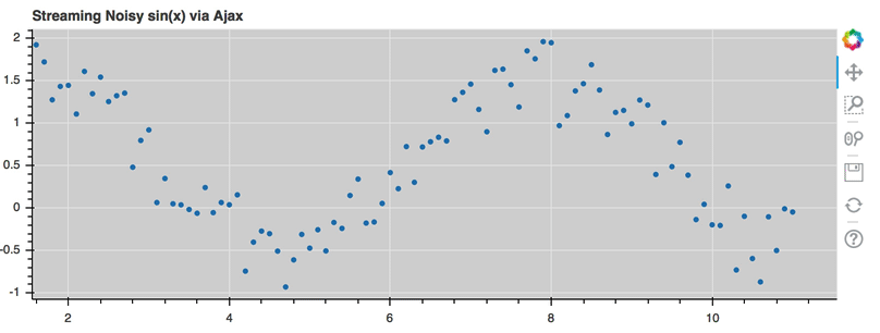
AjaxDataSource#

Updating and streaming data works very well with Bokeh server applications. However, it is also possible to use similar functionality in standalone documents. The AjaxDataSource provides this capability without requiring a Bokeh server.

To set up an AjaxDataSource, you need to configure it with a URL to a REST endpoint and a polling interval.

In the browser, the data source requests data from the endpoint at the specified interval. It then uses the data from the endpoint to update the data locally.

Updating data locally can happen in two ways: either by replacing the existing local data entirely or by appending the new data to the existing data (up to a configurable max_size). Replacing local data is the default setting. Pass either "replace" or "append"``as the AjaxDataSource's ``mode argument to control this behavior.

The endpoint that you are using with your AjaxDataSource should return a JSON dict that matches the standard ColumnDataSource format, i.e. a JSON dict that maps names to arrays of values:

{
    'x' : [1, 2, 3, ...],
    'y' : [9, 3, 2, ...]
}

Alternatively, if the REST API returns a different format, a CustomJS callback can be provided to convert the REST response into Bokeh format, via the adapter property of this data source.

Otherwise, using an AjaxDataSource is identical to using a standard ColumnDataSource:

# setup AjaxDataSource with URL and polling interval
source = AjaxDataSource(data_url='http://some.api.com/data',
                        polling_interval=100)

# use the AjaxDataSource just like a ColumnDataSource
p.circle('x', 'y', source=source)

This is a preview of what a stream of live data in Bokeh can look like using AjaxDataSource:

Animated image showing a timeseries scatter plot updating periodically via the ajax streaming data source.

For the full example, see examples/basic_data/ajax_source.py in Bokeh’s GitHub repository.

Linked selection#

You can share selections between two plots if both of the plots use the same ColumnDataSource:

from bokeh.layouts import gridplot
from bokeh.models import ColumnDataSource
from bokeh.plotting import figure, show
from bokeh.sampledata.penguins import data
from bokeh.transform import factor_cmap

SPECIES = sorted(data.species.unique())

TOOLS = "box_select,lasso_select,help"

source = ColumnDataSource(data)

left = figure(width=300, height=400, title=None, tools=TOOLS,
              background_fill_color="#fafafa")
left.scatter("bill_length_mm", "body_mass_g", source=source,
             color=factor_cmap('species', 'Category10_3', SPECIES))

right = figure(width=300, height=400, title=None, tools=TOOLS,
               background_fill_color="#fafafa", y_axis_location="right")
right.scatter("bill_depth_mm", "body_mass_g", source=source,
              color=factor_cmap('species', 'Category10_3', SPECIES))

show(gridplot([[left, right]]))

Linked selection with filtered data#

Using a ColumnDataSource, you can also have two plots that are based on the same data but each use a different subset of that data. Both plots still share selections and hovered inspections through the ColumnDataSource they are based on.

The following example demonstrates this behavior:

The second plot is a subset of the data of the first plot. The second plot uses a CDSView to include only y values that are either greater than 250 or less than 100.
If you make a selection with the BoxSelect tool in either plot, the selection is automatically reflected in the other plot as well.
If you hover on a point in one plot, the corresponding point in the other plot is automatically highlighted as well, if it exists.

from bokeh.layouts import gridplot
from bokeh.models import BooleanFilter, CDSView, ColumnDataSource
from bokeh.plotting import figure, show

x = list(range(-20, 21))
y0 = [abs(xx) for xx in x]
y1 = [xx**2 for xx in x]

# create a column data source for the plots to share
source = ColumnDataSource(data=dict(x=x, y0=y0, y1=y1))

# create a view of the source for one plot to use
view = CDSView(filter=BooleanFilter([True if y > 250 or y < 100 else False for y in y1]))

TOOLS = "box_select,lasso_select,hover,help"

# create a new plot and add a renderer
left = figure(tools=TOOLS, width=300, height=300, title=None)
left.circle('x', 'y0', size=10, hover_color="firebrick", source=source)

# create another new plot, add a renderer that uses the view of the data source
right = figure(tools=TOOLS, width=300, height=300, title=None)
right.circle('x', 'y1', size=10, hover_color="firebrick", source=source, view=view)

p = gridplot([[left, right]])

show(p)

Other data types#

You can also use Bokeh to render network graph data and geographical data. For more information about how to set up the data for these types of plots, see Network graphs and Geographical data.