Abstract Rendering
Abstract rendering is a bin-based rendering technique
that provides greater control over a visual representation
and access to larger data sets through server-side processing.
There are two interfaces for abstract rendering in Bokeh:
(1) a high-level Recipes Interface that provides common abstract rendering
configurations with good defaults and only optional parameterization
and (2) a low-level Functions Interface that provides access to the details
of the abstract rendering process.
The recipes interface actually produces elements in the low-level
interface, but through a level of indirection to simplify construction.
At a high level, all abstract rendering applications start with a plot.
Abstract rendering takes the plot and renders it to a canvas that uses
data values instead of colors and bins instead of pixels. With the data
values collected into bins, the plot can be analyzed and transformed to
ensure the true nature of the underlying data source is preserved.
This second step is referred to as ‘shading’
(older versions of abstract rendering called this step ‘transfer’,
but the current version is more general and thus the name change).
The abstract rendering interfaces take an existing Bokeh plot as a parameter.
They produce binning and shading processes, which are attached to a data source.
They also produce a new plot to consume the results of the shading.
and produce a new plot. By default, the old plot is removed.
Abstract rendering is tied to the bokeh server infrastructure, and can
thus only be used with an active bokeh server and with plots employing
a ServerDataSource.
Note
Because abstract rendering relies on server-side processing, it will only
work with bokeh server.
Note
Because abstract rendering uses some functions from the scipy.misc
module in its internal machinery, you need to install PIL (or Pillow) to make
it work. These libraries are not a dependency of SciPy and therefore, in general,
some of the functions from this module are not available on systems that don’t
have PIL (or Pillow) installed.
Abstract rendering recipes provide simplified access to common abstract
rendering operations. The recipes interface is declarative,
in that a high-level operation is requested and the abstract rendering
system constructs the proper low-level function combinations.
Abstract rendering recipe usage can be found
in census.py and abstractrender.py (in examples/plotting/server).
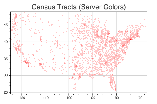
Heatmap converts a plot of points into a plot of densities.
The most common scenario is a recipes with one item type and overplotting issues.
Adjacency-matrix based graph visualizations also benefit from a heatmap if there is more than one node per pixel row/col.
The basic process is that each bin collects the count of the number of items
that fall into the bin. After that, a color scale is constructed that ensures
the full range of the data covers is covered by the color scale.
Heatmap is applicable when there is only one category and when the spatial
distribution of items is of interest. In many ways, it is a replacement for
alpha composition, but more flexible. It should be used when the dynamic
range of color composition of the visualization is essential to interpretation.
The color scale can be perceptually corrected
and include a large step from zero items to many (to ensure visibility of outliers).
Example heatmap:
source = ServerDataSource(data_url="/defaultuser/CensusTracts.hdf5",
                          owner_username="defaultuser")
plot = square( 'LON', 'LAT', source=source)
ar.heatmap(plot, spread=3, title="Census Tracts (Server Colors)")
Heatmap can be controlled with the following parameters:
- spread — Spread values out after binning. This is used for post-projection shapes.
- transform — Modify counts before building the color ramp?
Valid options include cbrt (default),``log`` and none.
- low — Color for the least dense bin in server coloring (excluding 0).
- high — Color for the most dense bin in server coloring.
- client_colors — If set to true, low/high are ignored and coloring is passed off to the client code.
- palette — Colors to use if client_colors is true
- Parameters understood by ‘replot’ in the functions interface may also be used
(thus ‘title’ in the example).
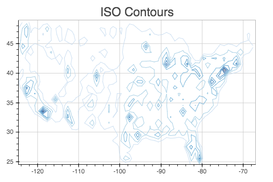
The contours recipe converts a plot of points into ISO contours.
It works on the same principal as the heatmap recipe (binning counts),
but instead of building color ramps, the contours recipe produces
a number of regions representing ranges of counts.
Using the same source plot as in heatmap, contours is applied like this:
colors = ["#C6DBEF", "#9ECAE1", "#6BAED6",
          "#4292C6", "#2171B5", "#08519C", "#08306B"]
ar.contours(plot, palette=colors, title="ISO Contours")
The contours recipe uses the following parameters:
- Palette — List of colors for each contour, in the desired order.
- Parameters understood by ‘replot’ in the functions interface may also be used.
HDAlpha converts a plot of points into a plot of densities, just like heatmap.
However, heatmap is restricted to a single category, while hdalpha works with multiple categories of data.
The hdalpha recipe is useful for scatterplots with multiple categories or
geo-located event data where events are of different types.
In the hdalpha recipe, categories are binned separately and a color ramp is made for each category.
Additionally, the composition between categories is also controlled to prevent over-saturation.
Example application of hdalpha:
source = ServerDataSource(data_url="fn://gauss", owner_username="defaultuser")
plot = square('oneA', 'oneB', color='cats', source=source)
ar.hdalpha(plot, spread=5, title="Multiple categories")
The parameters for hdalpha are the same as for contours, except
that palette determines the number categories instead of the number
of contours. If more categories are found than colors provided,
all additional categories are combined into the last category.
The functional interface for abstract rendering provides a set of building blocks for
creating and performing analysis on binned values. In this interface, you have the
opportunity to specify the steps of any analysis and full control over the parametrization.
In exchange, an understanding of the control flow and execution model in abstract rendering
is required.
Abstract rendering is configured via the ‘replot’ function.
Replot takes a plot and an abstract rendering configuration as arguments
and produces a new plot. It is the primitive which the recipes rely on
(in fact, extra arguments passed to recipes will be sent to replot).
The abstract rendering configuration breaks down into four function roles.
The function roles are:
- selector — Determines which bins are associated with a glyph in the visualization
- info — Determines which value goes into the bin for a given glyph
- aggregator — Combines new values (from info) with the existing value of the bin
- shader — Transforms a set of bins. Shaders may be chained in many cases.
In replot, the selector is determined either indirectly through the plot or via
the points flag. If points is set, then all geometry of the plot is interpreted
as points that touch only one bin. Otherwise, the shape-type of the source plot
will be used.
The info function refers back to the data source of the original plot. The row
related to the current shape is used as its argument. Since counts are common,
the default info function is Const(1), which always returns the value 1.
The info function is commonly used for categorization of the input glyphs.
The aggregator builds bin values from info values and an existing bin.
Count and CountCategories are the current aggregators.
Shaders transform sets of bins. The most common target is a new set of bins.
The output set of bins may be anything, though numbers and colors
are the most common. Shader chains that end in grids of numbers rely
on the BokehJS client to do coloring. Any chain that results in a grid of bins can be
extended with additional shaders. In contrast, the Contours shader produces sets of lines
instead of a new grid of bins.
Here is a re-creation of the heatmap recipe using the functions interface:
source = ServerDataSource(data_url="/defaultuser/CensusTracts.hdf5",
                          owner_username="defaultuser")
plot = square( 'LON', 'LAT', source=source)
ar.replot(plot,
          info=ar.Const(val=1),
          agg=ar.Count(),
          shader=ar.Spread(factor=3)
                   + ar.Cuberoot()  # Approximates perceptual correction
                   + ar.InterpolateColor(low=(255,200,200), high=(255,0,0)),
          points=True,
          reserve_val=0)
The list of available functions
and their relevant parameters is growing all the time. Please see
the docstrings for details. The above example is also found
in abstractrender.py (in examples/plotting/server).
Abstract rendering is also an active research project. If you would like more
information, the follow publications provide information on the experimental system
and the capabilities that may eventually be included in Bokeh through abstract rendering.
- Abstract rendering fully supports circle and square glyph types
in scatter plots. More complex shapes and lines cannot
used in the input plot at this time.
- If a plot is constructed with multiple layers, only the first layer using a ServerDataSource
can use abstract rendering.